Generalized Additive Model(GAM)
Zarathu Co.,Ltd
2022-09-25
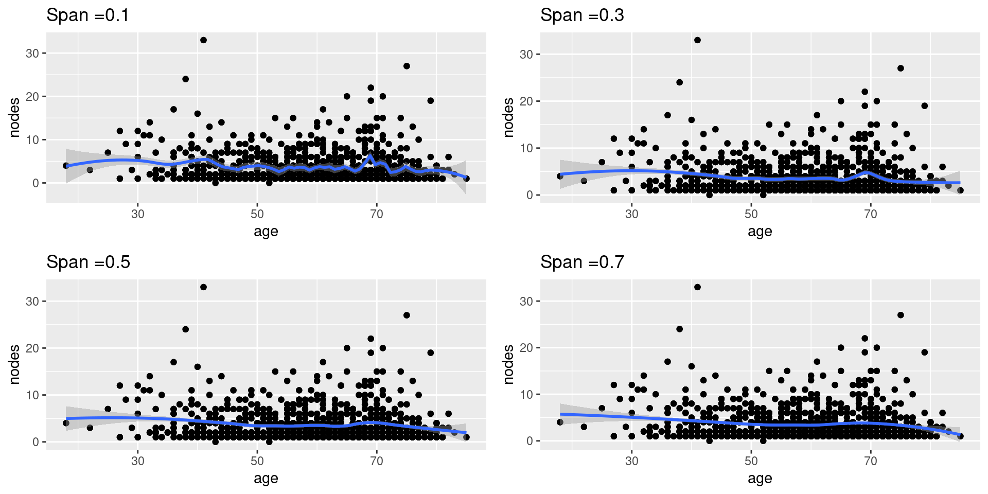
LOWESS
Locally weighted scatterplot smoothing
- 구간 나눠 regression
- 각 점마다 그 점을 포함하는 구간 설정
- 가까운 점에 weight

LOWESS in ggplot
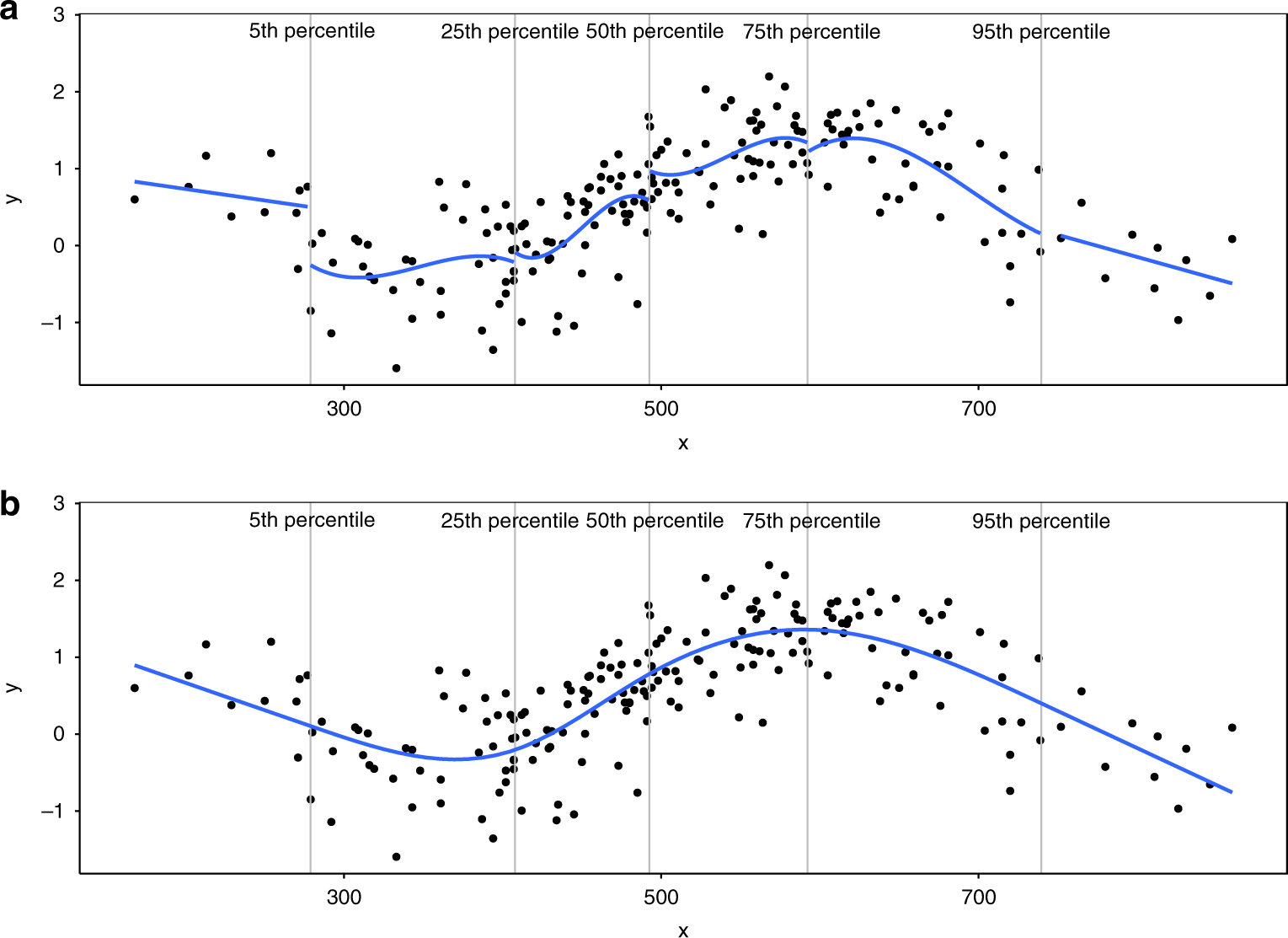
Cubic spline
Cubic = 3차방정식
- 구간을 몇 개로 나누고: knot
- 각각을 3차함수로 fitting
- 구간 사이 부드럽게 연결되도록 제한조건
Cubic spline in R
library(splines)
cs1 <- glm(time ~ bs(age, knots = c(40, 50, 60, 70)) + sex, data = colon)
cs2 <- glm(time ~ bs(age, df = 4) + sex, data = colon)
ns1 <- glm(time ~ ns(age, knots = c(40, 50, 60, 70)) + sex, data = colon)
ns2 <- glm(time ~ ns(age, df = 4) + sex, data = colon)

age.grid <- seq(min(colon$age), max(colon$age), by = 1)
with(colon, plot(age,time,col="grey",xlab="Age",ylab="Time"))
points(age.grid, predict(cs1, newdata = data.frame(age=age.grid, sex = 1)), col=1, lwd=1, type="l")
points(age.grid, predict(cs2, newdata = data.frame(age=age.grid, sex = 1)), col=2, lwd=2, type="l")
points(age.grid, predict(ns1, newdata = data.frame(age=age.grid, sex = 1)), col=3, lwd=3, type="l")
points(age.grid, predict(ns2, newdata = data.frame(age=age.grid, sex = 1)), col=4, lwd=4, type="l")
#adding cutpoints
abline(v = c(40, 50, 60, 70), lty=2, col="black")
legend("topleft", c("cs:knots" ,"cs:df", "ns:knots", "ns:df"), col = 1:4, lwd = 1:4)
\(\lambda\)
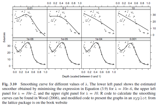
Plot
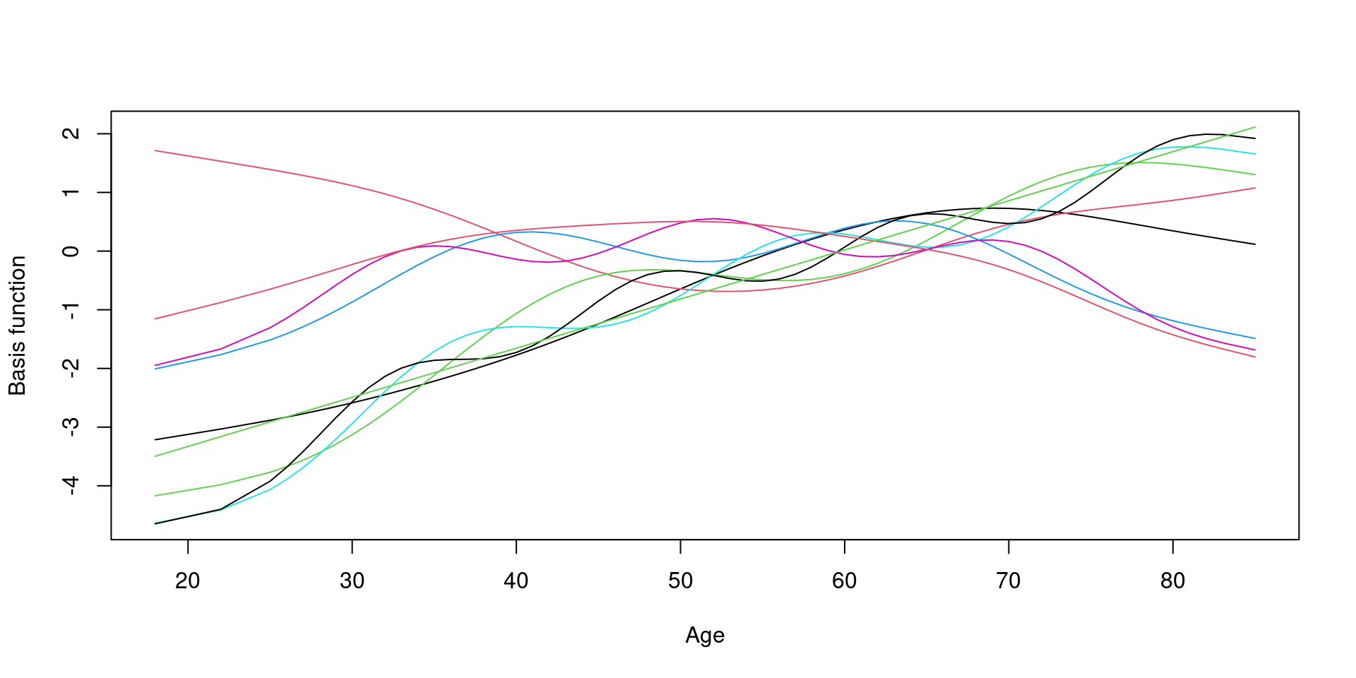
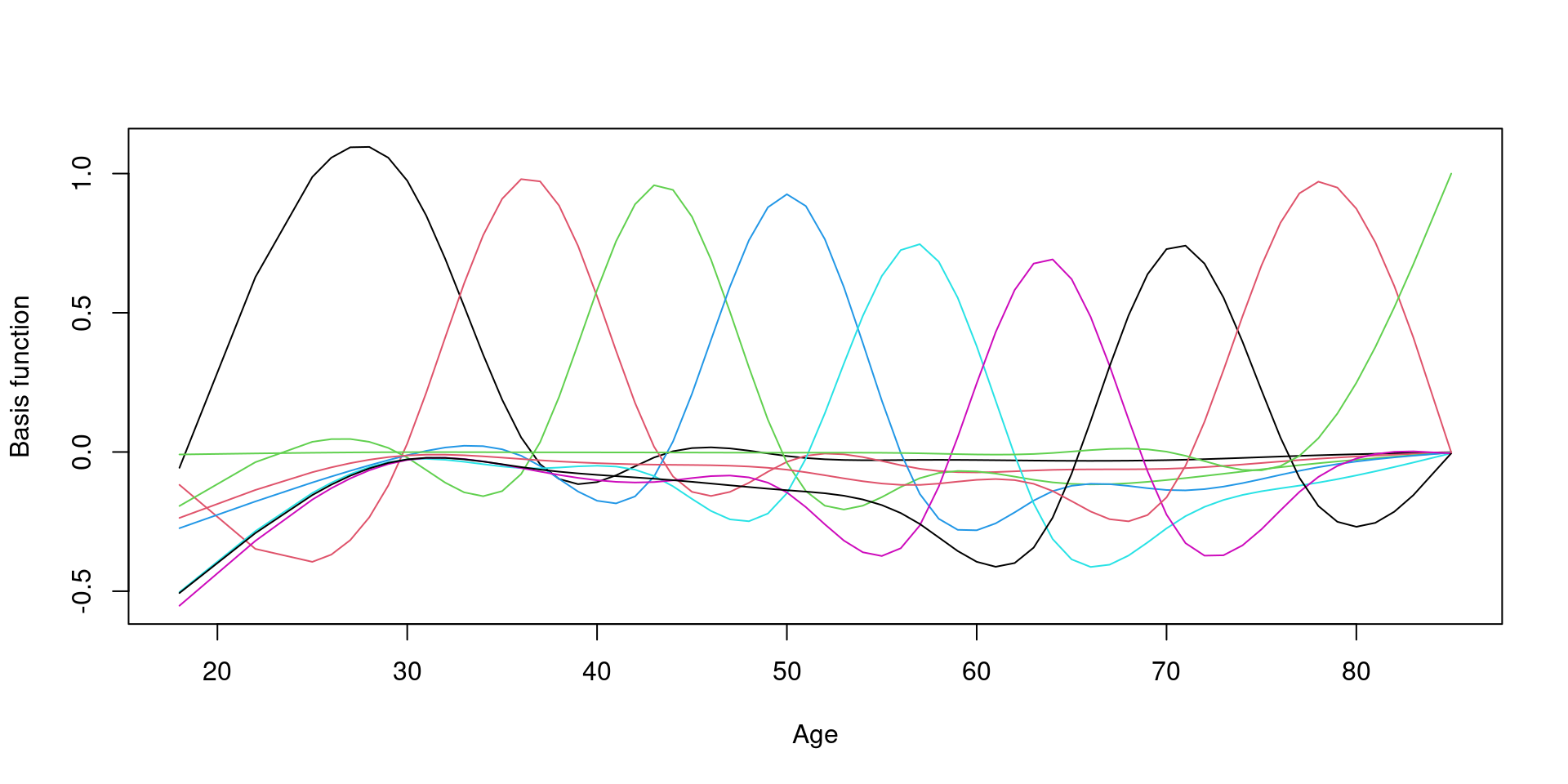
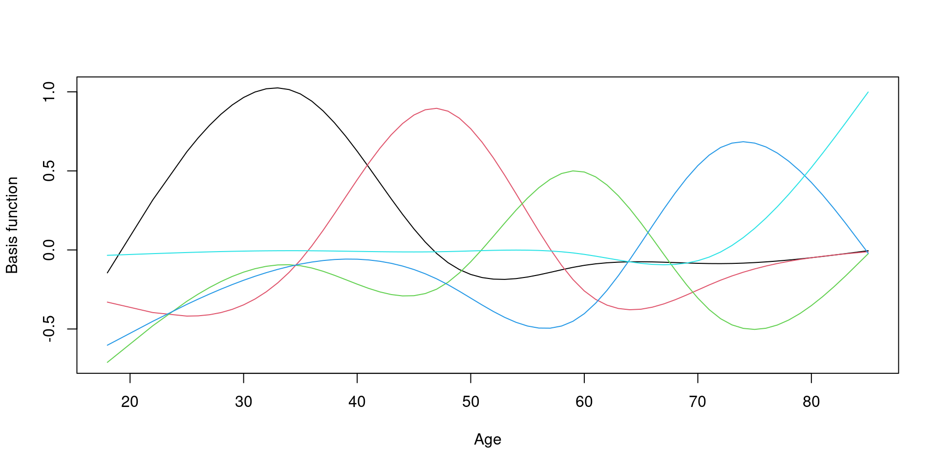
Basis function
Smoothing spline: basis function 들의 합
\[s(x) = \sum_{k = 1}^K \beta_k b_k(x)\]
Basis function: plot
9개의 basis function
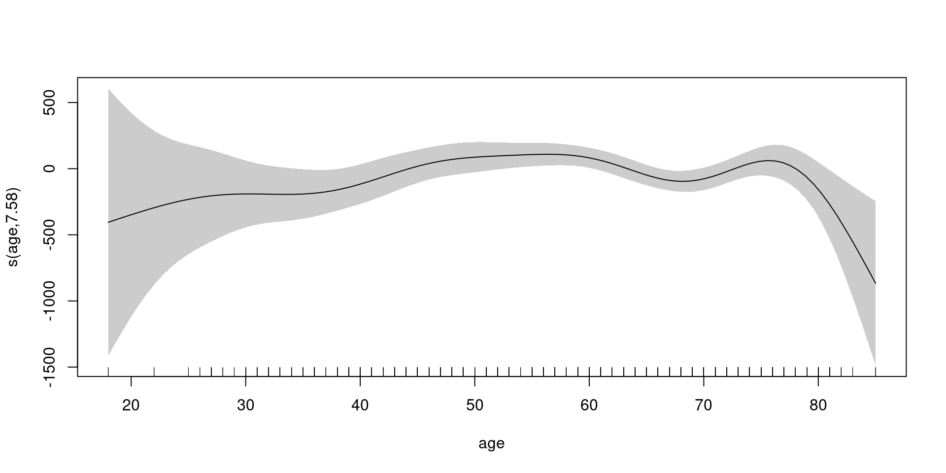
GAM result
model_matrix 에 계수를 곱하면 곡선의 y값
 (Intercept)          sex     s(age).1     s(age).2     s(age).3     s(age).4
 1533.193607     8.353593   776.245594  1393.793067   232.785846 -1154.982151
    s(age).5     s(age).6     s(age).7     s(age).8     s(age).9
324.817013 -1018.225598 274.926370 3106.242791 -783.531680 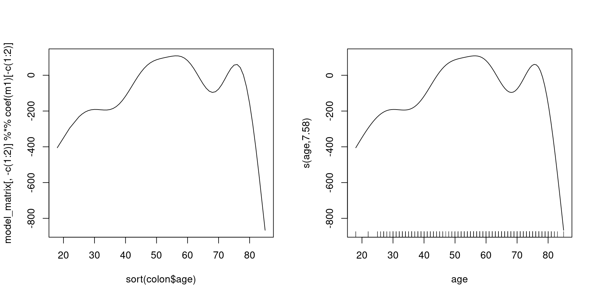
Change basis function
Restricted df
\(k = 6\): df의 최대값을 6으로 제한
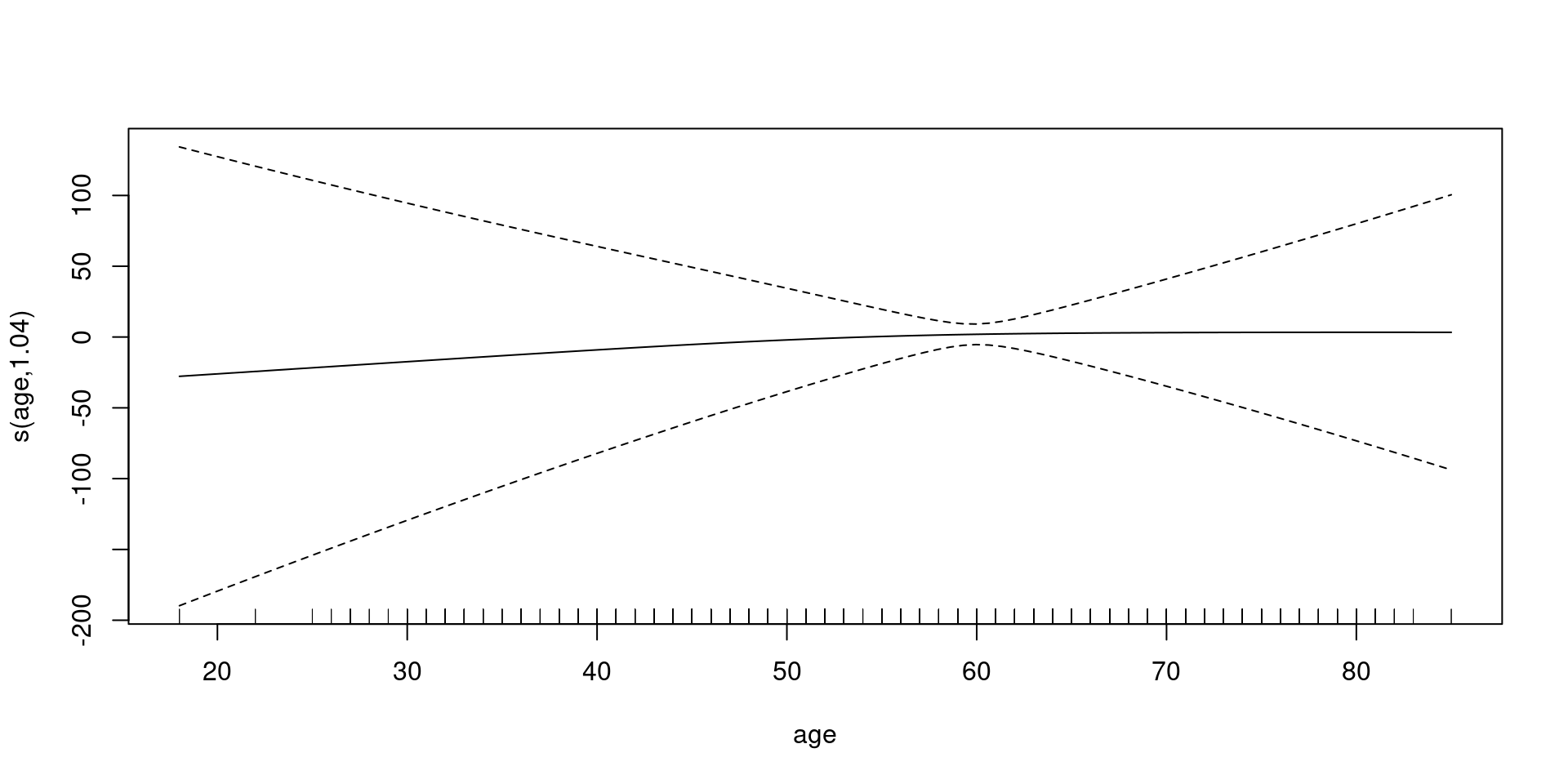
Fix \(\lambda\)
sp = 1000: \(\lambda\) 1000으로 고정, 거의 직선을 의미
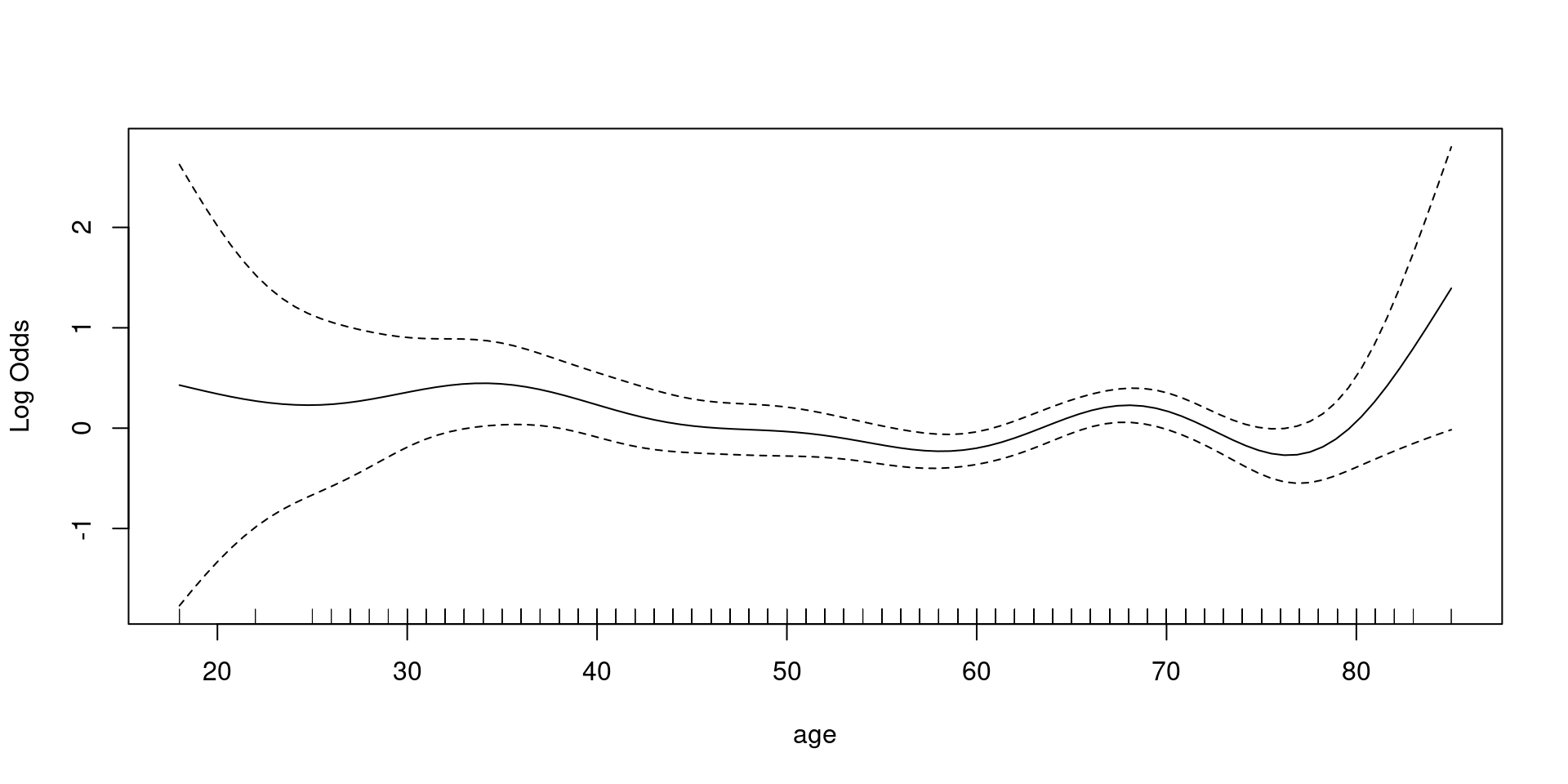
Logistic
family = binomial
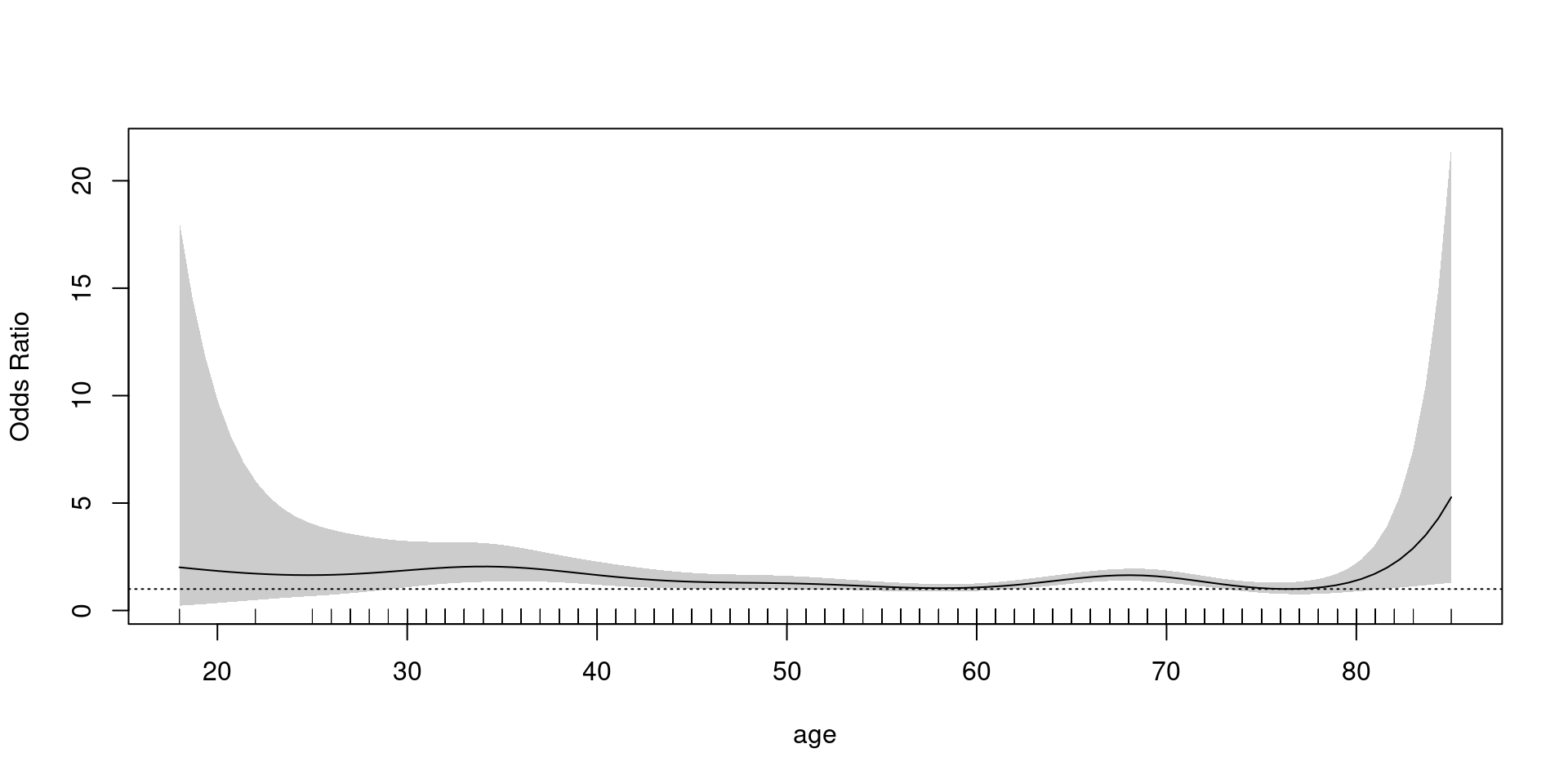
- 해석에 주의: log Odds
- exponential transformation, reference(OR =1) 설정 필요
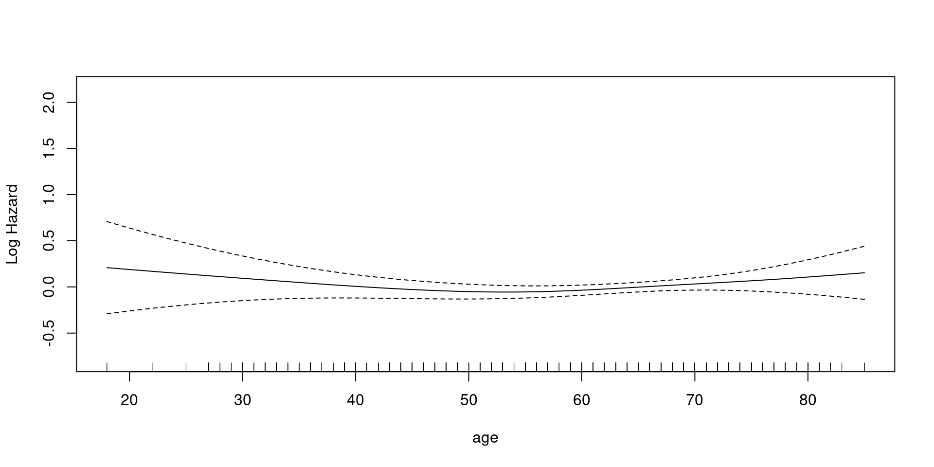
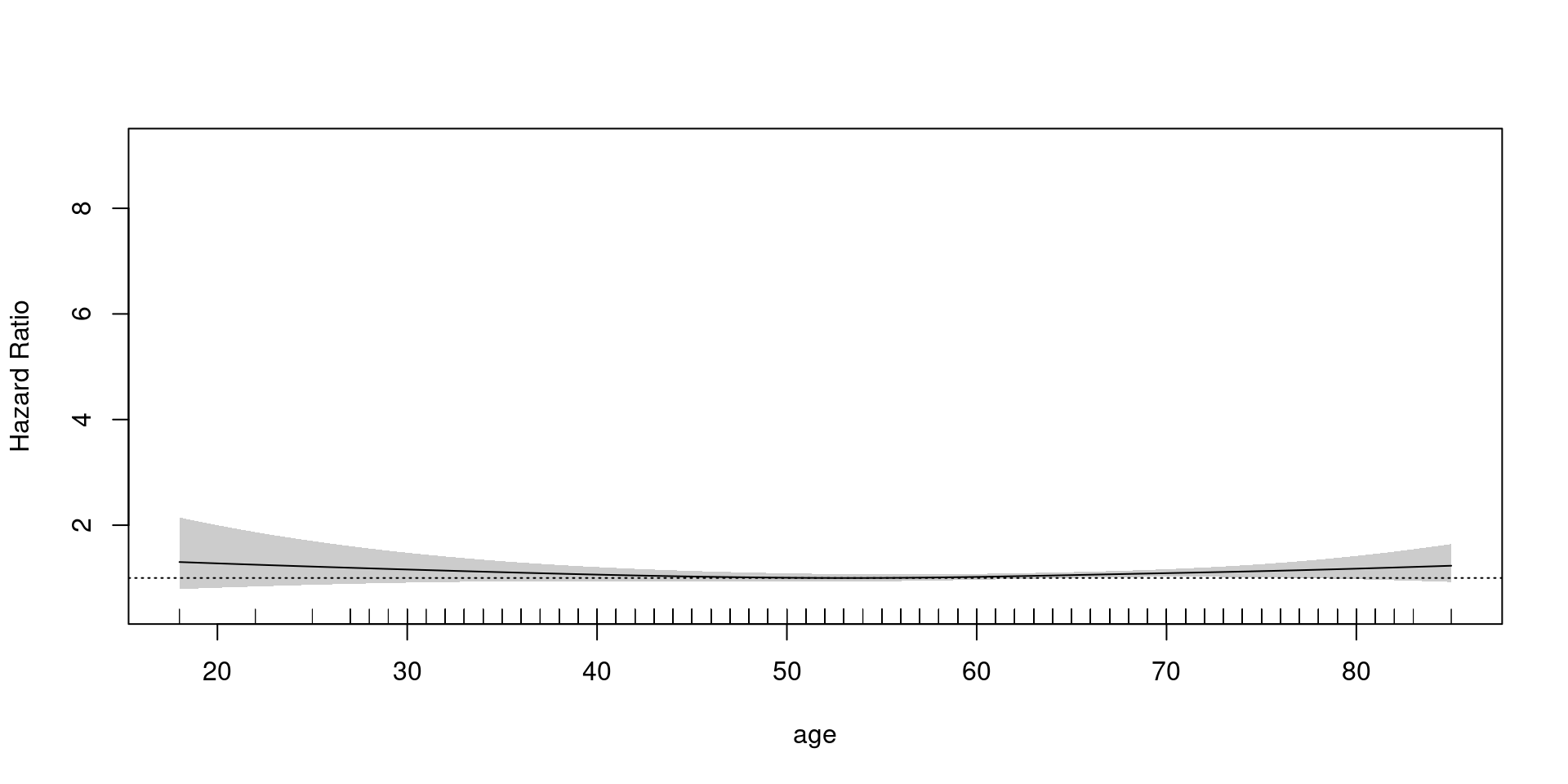
Coxph
family = cox.ph - weights = status
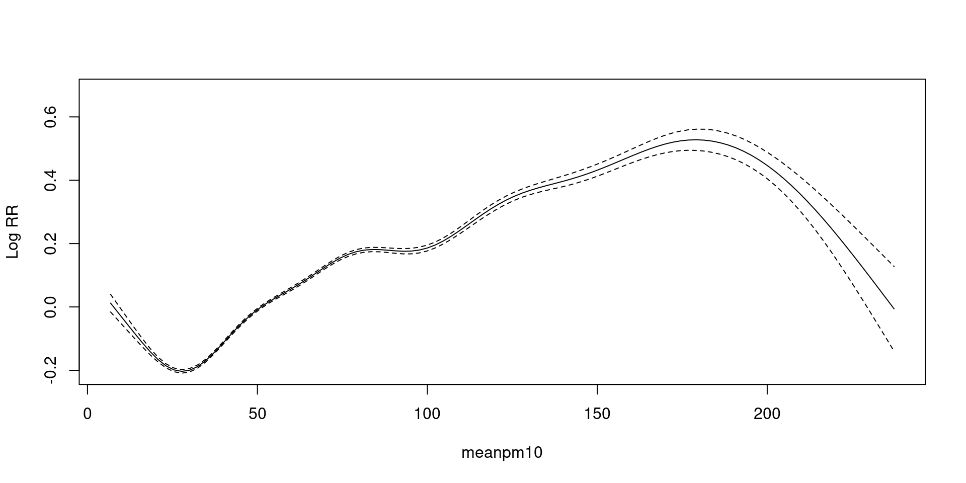
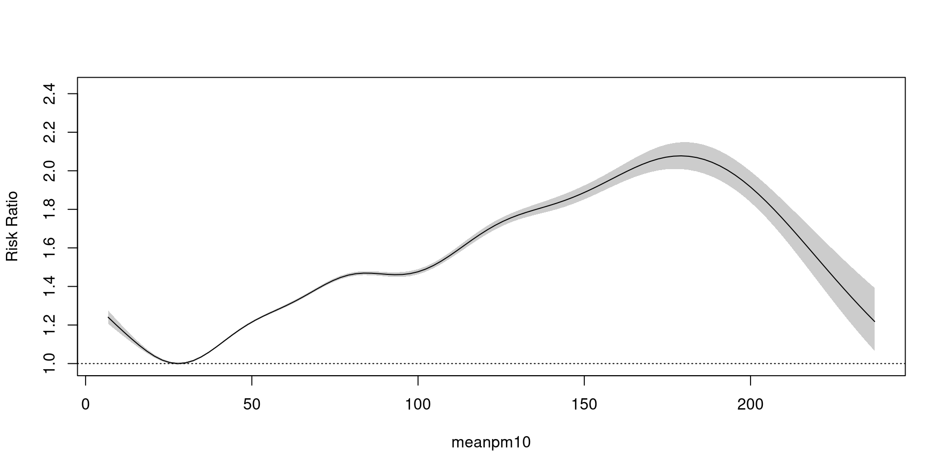
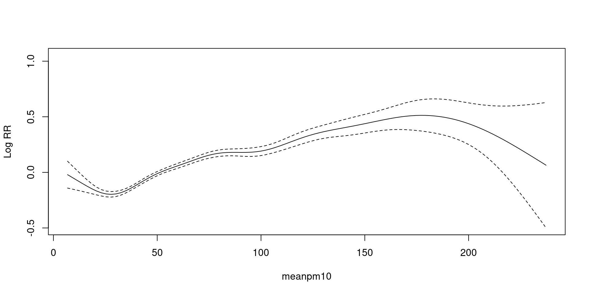
Poisson
family = poisson - exp trans
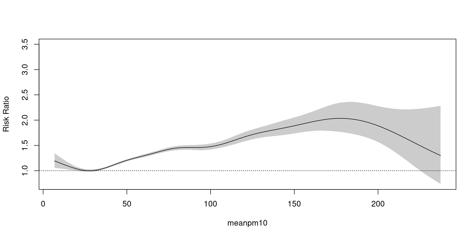
Quasi-poisson
Poisson 분포의 가정 평균=분산 이 만족하지 않을 때.
family = quasipoisson- \(평균 = \phi * 분산\)
- 곡선 자체는 그대로, 신뢰구간만 넓어짐(보수적 추정)
Thank you for your time