Regression and
Survival Analysis

Zarathu

Executive Summary

	Default	Repeated Measure	Survey
Continuous	Linear regression	GEE	Survey GLM
Event	GLM (logistic)	GEE	Survey GLM
Time & Event	Cox	Marginal Cox	Survey Cox
0,1,2,3 (rare event)	GLM (Poisson)	GEE	Survey GLM

Practice Dataset

Linear regression

Continuous

Simple

\[Y = \beta_0 + \beta_1 X + \epsilon\] Estimate $\beta_0$, $\beta_1$ by minimizing sum of squared errors

$Y$ must be continuous & normally distributed
$X$ can be continuous or categorical
- If continuous: same as correlation analysis
- If binary: same as t-test with equal variance

Bivariate Correlation

Use the Bivariate Correlation function to test linear association between two continuous variables.

Analyze → Correlate → Bivariate…

Move age and nodes into the Variables box
Select Pearson as the correlation coefficient
Choose Two-tailed test of significance

Pearson correlation: r = -0.093
p-value: < .001 → statistically significant
Sample size: N = 1822

There is a weak negative, yet statistically significant, correlation between age and nodes.

Linear Regression: Predicting Nodes from Age

This regression estimates how age affects nodes (number of affected lymph nodes).

Go to Analyze → Regression → Linear…

Set nodes as the Dependent variable and age as the Independent(s) variable.

R = .093, R² = .009: Very weak linear relationship
Unstandardized coefficient for age = -0.028, p < .001

As age increases by 1 year, the number of nodes is expected to decrease by 0.028. The relationship is statistically significant but weak.

Linear Regression: Predicting Age from Nodes

This reverses the regression direction, predicting age from nodes.

Go to Analyze → Regression → Linear…
Set age as the Dependent variable and nodes as the Independent(s) variable.

R = .093, R² = .009: Same strength as the previous model (symmetric)
Unstandardized coefficient for nodes = -0.309, p < .001

Although both models are statistically significant (p < .001), the effect size (R² ≈ 0.009) is very small. This indicates that only about 0.9% of the variance in either variable is explained by the other.

T-tests & Simple Linear Regression

are equivalent when comparing 2 groups

Independent Samples T-test: Comparing Time by Sex

To compare the variable time between male and female groups using a t-test in SPSS:

t = -0.317, df = 1856, p = 0.751
No statistically significant difference in mean time between groups

We begin with a t-test because it is a simple, standard method for comparing group means when the predictor has only two levels. It provides the same result as regression but is more intuitive in this context.

Simple Linear Regression: Predicting Time from Sex

This analysis fits a linear regression model where time is predicted by sex.

Go to Analyze → Regression → Linear…
Set time as the Dependent variable and sex as the Independent(s) variable.

The regression result is consistent with the t-test:

There is no statistically significant association between sex and time.

More than 2 Groups?

Changing string into numeric in SPSS

The variable rx includes three treatment groups:
- 1 = Lev
- 2 = Lev+5FU - 3 = Obs (reference)

In SPSS, linear regression does not automatically treat string variables as categorical. To include a categorical variable like rx in a regression model, we must first convert it to numeric.

Use Automatic Recode if your original rx is a string variable. This assigns numeric values starting from 1: 1 = Lev, 2 = Lev+5FU, 3 = Obs

If it is a numeric variable, SPSS automatically chooses the lowest numeric value as the reference category.

This will assign numeric values starting from 1.

Now that rx_new is numeric, SPSS will automatically create dummy variables when used in regression BUT it will use the lowest number as the reference group (e.g., 1 = Lev). To change the reference group (e.g., set 3 = Obs), go to Categorical… and select it manually.

Linear Regression with Categorical Variables (3 Groups)

Go to Transform → Compute Variable… To include a 3-group variable in regression, create two dummy variables:
- rx_lev = 1 if rx_new == 1, else 0
- rx_lev5fu = 1 if rx_new == 2, else 0

The reference group (row where all dummy variables are 0) is Obs, which is not coded explicitly.

Use Analyze → Regression → Linear

Dependent variable: time
Independent variables: rx_lev, rx_lev5fu

The constant is the mean for the Obs group. Coefficients show the difference from Obs: - rx_lev = difference between Lev and Obs
- rx_lev5fu = difference between Lev+5FU and Obs

Only rx_lev5fu shows a significant difference (p < .001)

Alternative: One-Way ANOVA

Use Analyze → Compare Means → One-Way ANOVA
to test whether any of the rx_new groups differ overall. - Dependent = time
- Factor = rx_new

Options → Check Homogeneity of variance test (Levene’s test)

This gives an overall p-value for overall group comparison.

Multiple Variables

Including multiple variables

\[Y = \beta_0 + \beta_1 X_{1} + \beta_2 X_{2} + \cdots + \epsilon\]

Interpretation of $\beta_1$: When adjusting for $X_2$, $X_3$, etc., a one-unit increase in $X_1$ leads to an increase of $\beta_1$ in $Y$.

In academic papers,

it is common to present results both before and after adjustment.

Unadjusted Analyze each variable one at a time:

Go to Analyze → Regression → Linear
Set time as Dependent
Add one predictor (e.g., sex) to Independent(s)

Adjusted Control for multiple variables:

Set time as Dependent
Add all predictors (e.g., sex, age, rx) to Independent(s)

This allows comparison of crude vs. adjusted effects.

Logistic regression

Used for Binary Outcomes: 0/1

\[ P(Y = 1) = \frac{\exp{(X)}}{1 + \exp{(X)}}\]

Odds Ratio

\[ \begin{aligned} P(Y = 1) &= \frac{\exp{(\beta_0 + \beta_1 X_1 + \beta_2 X_2 + \cdots)}}{1 + \exp{(\beta_0 + \beta_1 X_1 + \beta_2 X_2 + \cdots)}} \\\\ \ln(\frac{p}{1-p}) &= \beta_0 + \beta_1 X_1 + \beta_2 X_2 + \cdots \end{aligned} \]

Interpretation of $\beta_1$: When adjusting for $X_2$, $X_3$, etc., a one-unit increase in $X_1$ results in an increase of $\beta_1$ in $\ln\left(\frac{p}{1 - p}\right)$ (the log-odds of the outcome).

$\frac{p}{1-p}$ increases by a factor of $\exp(\beta_1)$. In other words, the odds ratio = $\exp(\beta_1)$.

Finding Odds Ratio in SPSS

Go to Analyze → Regression → Binary Logistic... Move status to the Dependent box, sex, age, and rx_new into the Covariates box.

Click Categorical…
Select rx_new, move to Categorical Covariates
Set Reference Category to Last (e.g., Obs)

Exp(B) gives odds ratios

Cox proportional hazard

Time & Event

Time to event data

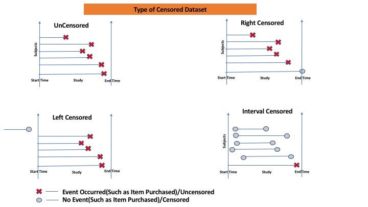
Most data are right-censored: the individual either died on day XX or survived up to day XX.

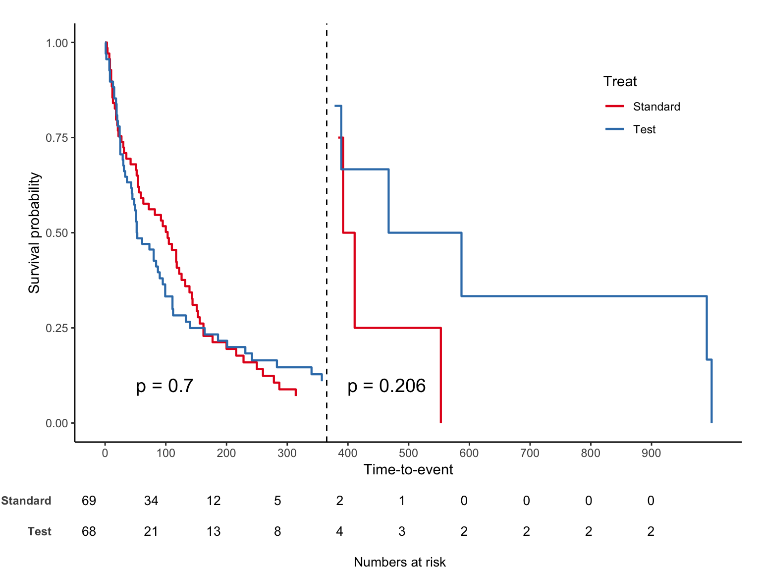
Representing Time-to-Event with One Variable

Kaplan-meier plot

In survival analysis, Table 1 typically presents baseline characteristics.

It is usually accompanied by the log-rank test p-value to compare survival between groups.

Go to Analyze → Survival → Kaplan-Meier…
Set time as Time, status(1) as Status, rx_new as Factor

Click Options → Check:

Survival table(s)
Mean and median survival
Survival plot

Click Compare Factor… → Check:

Log rank
Pooled over strata

Click OK to see:

Kaplan–Meier plot with censored cases (+)
Log-rank p-value comparing survival curves

Calculation:

Sort by time in ascending order

\[ \begin{aligned} P(t) &= \frac{\text{Survived at } t}{\text{At risk at } t} \quad \text{(Interval survival)} \\\\ S(t) &= S(t-1) \times P(t) \end{aligned} \]

Logrank test

Compute the expected number of events for each interval, then combine them for a chi-squared test.

Is it combining the results across intervals?

Assumes similar event patterns across intervals (proportional hazards assumption).

Cox model

Hazard function: $h(t)$

Probability of surviving up to time $t$ and dying immediately after

Cox model: evaluates the Hazard Ratio (HR)

\[ \begin{aligned} h(t) &= \exp({\beta_0 + \beta_1 X_1 + \beta_2 X_2 + \cdots}) \\\\ &= h_0(t) \exp({\beta_1 X_1 + \beta_2 X_2 + \cdots}) \end{aligned} \] When $X_1$ increases by 1, $h(t)$ increases by a factor of $(_1)$. In other words:

\[\text{HR} = \exp{(\beta_1)}\]

Characteristics

Like Kaplan-Meier, statistics are calculated by intervals.

Assumes similar patterns across intervals (proportional hazards assumption)

Time-independent HR: time is captured only by $h_0(t)$.

Model is simple: HR remains constant over time
Time-dependent Cox models are also possible

$h_0(t)$ is not estimated, which simplifies computation

This is why Cox is called a semi-parametric method
But it’s a limitation when building prediction models — you need to estimate $h_0(t)$ separately

Cox Regression in SPSS

Go to Analyze → Survival → Cox Regression

Set Time = time, Status = status
Click Define Event, enter value = 1

Move sex, age, rx_new to Covariates
Click Categorical, add rx_new, set Reference Category to Last, click Change
Exp(B) = hazard ratio

Survival Analysis:

Proportional Hazards Assumption

Assumes a consistent trend: survival curves should not cross - No formal test for the assumption is strictly required — it can be checked visually.

Landmark-analysis

Analyze separately by dividing time into intervals.

Time-dependent cox

Time-dependet cox

Call:
coxph(formula = Surv(tstart, time, status) ~ trt + prior + karno:strata(tgroup), 
    data = vet2)

  n= 225, number of events= 128 

                                  coef exp(coef)  se(coef)      z Pr(>|z|)    
trt                          -0.011025  0.989035  0.189062 -0.058    0.953    
prior                        -0.006107  0.993912  0.020355 -0.300    0.764    
karno:strata(tgroup)tgroup=1 -0.048755  0.952414  0.006222 -7.836 4.64e-15 ***
karno:strata(tgroup)tgroup=2  0.008050  1.008083  0.012823  0.628    0.530    
karno:strata(tgroup)tgroup=3 -0.008349  0.991686  0.014620 -0.571    0.568    
---
Signif. codes:  0 '***' 0.001 '**' 0.01 '*' 0.05 '.' 0.1 ' ' 1

                             exp(coef) exp(-coef) lower .95 upper .95
trt                             0.9890      1.011    0.6828    1.4327
prior                           0.9939      1.006    0.9550    1.0344
karno:strata(tgroup)tgroup=1    0.9524      1.050    0.9409    0.9641
karno:strata(tgroup)tgroup=2    1.0081      0.992    0.9831    1.0337
karno:strata(tgroup)tgroup=3    0.9917      1.008    0.9637    1.0205

Concordance= 0.725  (se = 0.024 )
Likelihood ratio test= 63.04  on 5 df,   p=3e-12
Wald test            = 63.7  on 5 df,   p=2e-12
Score (logrank) test = 71.33  on 5 df,   p=5e-14

Time-dependent covariate

In survival analysis, all covariates should be measured before the index date - e.g., F/U lab, medication

To handle time-dependent covariates, a Cox model that accounts for this is required

Executive Summary

	Dafault	Repeated measure	Survey
Continuous	linear regression	GEE	Survey GLM
Event	GLM (logistic)	GEE	Survey GLM
Time & Event	Cox	marginal Cox	Survey Cox
0,1,2,3 (rare event)	GLM (poisson)	GEE	Survey GLM

Regression and Survival Analysis

Executive Summary

Practice Dataset

Linear regression

Simple

Bivariate Correlation

Linear Regression: Predicting Nodes from Age

Linear Regression: Predicting Age from Nodes

T-tests & Simple Linear Regression

Independent Samples T-test: Comparing Time by Sex

Simple Linear Regression: Predicting Time from Sex

More than 2 Groups?

Changing string into numeric in SPSS

Linear Regression with Categorical Variables (3 Groups)

Alternative: One-Way ANOVA

Multiple Variables

Including multiple variables

In academic papers,

Logistic regression

Odds Ratio

Finding Odds Ratio in SPSS

Cox proportional hazard

Time to event data

Representing Time-to-Event with One Variable

Kaplan-meier plot

Calculation:

Logrank test

Cox model

Characteristics

Cox Regression in SPSS

Survival Analysis:

Landmark-analysis

Time-dependent cox

Time-dependet cox

Time-dependent covariate

Executive Summary

END

Regression and
Survival Analysis