Descriptive Statistics in Medical Research

Jinseob Kim

Zarathu

Executive Summary

• Comparison of two groups (continuous variables): If normality is assumed, use a t-test; otherwise, use the Wilcoxon test.

• Comparison of three or more groups (continuous variables): If normality is assumed, use one-way ANOVA; otherwise, use the Kruskal–Wallis one-way ANOVA.

• Comparison of categorical variables: If the sample size is sufficient, use the Chi-square test; otherwise, use the Fisher’s exact test.

What is Descriptive Statistics?

• Refers to the numbers that summarize data —such as the mean, median, variance, and frequency tables— and graphs such as histograms and box plots.

• However, instead of presenting simple descriptive statistics, most medical research focuses on comparing them across groups, as shown in Table 1 (ex: by sex or disease status).

Research Flow

1. Present the data using descriptive statistics
2. Test hypotheses using univariate analysis
3. Use multivariate or subgroup analysis to control for effects of other variables

• Many simple studies end with univariate analysis, which is essentially equivalent to comparing descriptive statistics across groups.

• Therefore, understanding the statistics required for Table 1 alone can be sufficient for conducting basic medical research.

Grouped Comparison of
Continuous Variables

2 Groups: T-test

Comparison of means between the two groups

• Requires the mean and standard deviation of each group.

• Can be performed directly at: T-test Calculator

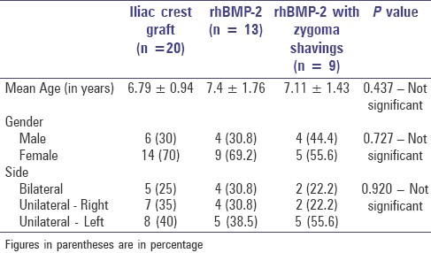
Data Table

T-test in SPSS

• Go to Analyze → Compare Means and Proportions → Independent-Samples T Test
• Test Variable: tChol
  
• Grouping Variable: sex (Female, Male)

T-test in SPSS

The mean difference in cholesterol (2.85) was not significant (p = .759 / .721) and the 95% CI included 0, indicating no difference between sexes.

• SPSS provides results for both cases: Equal variances assumed and not assumed.

• The second row (Welch’s t-test) is used when equal variances are not assumed.

• Assuming equal variances simplifies computation, but making this assumption without justification can be risky. Unless justified, use “Equal variances not assumed”.

• Running ANOVA on two groups is equivalent to a t-test assuming equal variances. There is also a version of ANOVA that does not assume equal variances.

Boxplot in SPSS

Go to Graphs → Boxplot….

Select Simple and Summaries for groups of cases, then click Define.

Set tChol as the Variable and sex as the Category Axis, then click OK.

The boxplot displays the distribution of cholesterol levels by sex.

Barplot in SPSS

Go to Graphs → Bar….

Select Simple and Summaries for groups of cases, then click Define.

Set tChol as the Variable (e.g., MEAN(tChol)) and sex as the Category Axis, then click OK.

The bar chart displays the mean cholesterol levels by sex.

2 Groups: Wilcoxon Test

When normality cannot be assumed: compare medians between two groups

• Uses rank information instead of raw values — a nonparametric test
• Results are typically presented as Median [IQR (25%–75% quantile)]

A formal normality test is not necessary to decide whether to use this method.

It is better to rely on clinical judgment.
For example, height and weight often follow a normal distribution,
while CRP levels or number of children typically do not.

• Reference for Normal Distribution

Wilcoxon Test in SPSS

Go to Transform → Automatic Recode….

Select the string variable sex to recode, and enter a new name like sex_num in the New Name field.

Click Add New Name then OK. SPSS will automatically assign numeric codes 'Male' → 1 and 'Female' → 2.

Go to Analyze → Nonparametric Tests → Legacy Dialogs → 2 Independent Samples….

Set tChol as the Test Variable and sex_num as the Grouping Variable, then click Define Groups and enter 1 and 2.

The output provides the Mann–Whitney U test results, including ranks and p-value.

3 or More Groups: One-way ANOVA

Comparison of means across three or more groups

• ANOVA tests whether at least one group differs significantly from the others overall.
• It tells you if there is a difference, but not which groups are different (run post-hoc analysis to determine which groups differ).

The standard ANOVA assumes equal variances across all groups, and when comparing only two groups, it produces the same result as a t-test assuming equal variances.

There is also a generalized ANOVA that does not assume equal variances, and our institution uses this as the default.

Standard ANOVA in SPSS

Standard ANOVA in SPSS

Go to Transform → Automatic Recode….

Select the string variable group to recode, and enter a new name like group_num in the New Name field.

Click Add New Name then OK. SPSS will automatically assign numeric codes 'A' → 1, 'B' → 2, 'C' → 3.

Go to Analyze → Compare Means and Proportions → One-Way ANOVA….

Set tChol as the Dependent List and group_num as the Factor, then click OK.

The output displays the F-statistic, p-value, and effect sizes such as eta-squared.

Generalized ANOVA in SPSS

Go to One-Way ANOVA… → Options… and check Welch test to account for unequal variances.

Use the \(p\)-value = 0.020 from unequal variance ANOVA, which indicates a statistically significant difference in total cholesterol among the three groups.

3 or More Groups: Kruskal–Wallis ANOVA

When normality cannot be assumed: compare medians across three or more groups

• Uses rank information instead of raw values — a nonparametric test

• Results are typically presented as Median [IQR (25%–75% quantile)]

Kruskal–Wallis Test in SPSS

Go to Analyze → Nonparametric Tests → Legacy Dialogs → K Independent Samples…

Move tChol into the Test Variable List and group_num into the Grouping Variable field.
Click Define Range… and enter minimum = 1, maximum = 3.

Click OK to run the test. The output will include rank comparisons and the Kruskal–Wallis H statistic.

Use the \(p\)-value = 0.025 from the Kruskal–Wallis test, which indicates a statistically significant difference in total cholesterol across the three groups.

Group Comparison of Categorical Variables

Much simpler than for continuous variables — no need to consider the number of groups or normality. The only thing to check is whether the sample size is sufficient.

Sufficient Sample Size:
Chi-square Test

The Chi-square test is used to determine whether two categorical variables are associated.

• It can also be applied to three or more categorical variables,
  but this lecture will not cover those cases.

Chi-square Test in SPSS

Chi-square Test in SPSS

At a glance, it’s hard to tell whether there is an association.
Let’s perform a Chi-square test to find out.

Chi-Square Test in SPSS

Go to Analyze → Descriptive Statistics → Crosstabs…

Set one variable HTN_medi as the Row(s) variable and another DM_medi as the Column(s) variable.
Click Statistics… and check Chi-square, then click Continue.

Click OK to run the test.

Use p-value = 0.474, which indicates that there is no statistically significant association between hypertension medication and diabetes medication use.

Insufficient Sample Size: Fisher’s Exact Test

When a category in the table being analyzed has a very small sample size, the Chi-square test becomes unreliable. In such cases, use Fisher’s Exact Test instead.

• Fisher’s test calculates the direct probability of observing a result as extreme or more extreme than the current one.

Fisher’s Exact Test in SPSS

Fisher’s Exact Test in SPSS

For this new dataset, let’s first try applying the Chi-squared test.

Since only 2 people are taking both medications, one of the cells in the contingency table has a very small sample size.

SPSS gives us the following warning: “1 cells (25.0%) have expected count less than 5. The minimum expected count is 2.20.” This violates the Chi-square test’s assumptions, making its result unreliable. In such cases, it’s better to use Fisher’s Exact Test, which does not rely on large sample approximations.

Fisher’s Exact Test in SPSS

Let’s try the Fisher’s exact test instead. The first steps are the same as for Chi-Square.

In Crosstabs…, go to Cells… then ensure Observed is checked under Counts.

Then, go to Exact… to check Exact to request Fisher’s Exact Test.

Fisher’s Exact Test indicated no statistically significant association between the two variables, p = 1.000 (2-sided).

Question: If Fisher’s test works in all cases, why not just always use it instead of the Chi-square test?

• When sample sizes are small, Fisher’s exact test is indeed simpler and methodologically sound. However, as sample size or the number of groups increases, the computational burden of Fisher’s test grows rapidly. Therefore, it is generally recommended to try the Chi-square test first.

Paired Group Comparison for Continuous Variables

2 Groups: Paired t-test

Suppose each person’s blood pressure was measured once manually and once using an automatic device.
Is a t-test sufficient to compare the two sets of measurements?

• A regular t-test calculates the mean of each method first and tests whether they are equal,
  which fails to utilize the paired nature of the data.

• A better approach is to first calculate the difference between the two measurements for each person,
  and then test whether the mean of these differences is zero.
  This method both uses the paired structure and is computationally simpler.

• The method of testing whether the mean of the differences is zero is called the paired t-test.

Paired Samples T-Test in SPSS

Paired Samples T-Test in SPSS

Go to Analyze → Compare Means → Paired-Samples T Test…

Select the two related variables (e.g., SBP_hand and SBP_machine) and move them into the Paired Variables box.

Interpret the Sig. (2-tailed) value in the output.

The test calculated the difference in SBP for each individual and then tested whether the mean of those differences was significantly different from zero, resulting in a p-value of 0.648.

Wilcoxon Signed-Rank Test

The nonparametric version of the paired t-test is the Wilcoxon signed-rank test,
which can be performed as follows:

Go to Analyze → Nonparametric Tests → Related Samples…

Select the two related variables (e.g., SBP_hand and SBP_machine) and move them into the Test Fields box under the Fields tab.

Go to the Settings tab, select Customize tests, and check Wilcoxon matched-pair signed-rank (2 samples).

Interpret the Asymptotic Sig. (2-sided) value in the output.

The test ranked the differences in SBP between hand and machine measurements for each individual and tested whether the median difference was significantly different from zero. The result was a p-value of 0.940 — there is no statistically significant difference.

• Although it will not be covered in this lecture, when comparing three or more paired groups, use repeated measure ANOVA.

Paired Group Comparison for Categorical Variables

McNemar Test, Symmetry Test for a Paired Contingency Table

2 Groups: McNemar Test

• Suppose we want to examine whether there is a difference in abdominal pain symptoms before and after taking a medication.
• The chi-squared test examines the overall association between abdominal pain before and after taking the medication, but it does not account for the fact that the data are paired (i.e., measured on the same individuals).
  
• To properly analyze paired data, we should use the McNemar test instead.

McNemar Test in SPSS

Go to Analyze → Descriptive Statistics → Crosstabs…

Set Pain_before as the Row(s) variable and Pain_after as the Column(s) variable. Click Statistics…, then check McNemar.

Click OK to run the test.

The McNemar test analyzes only the participants whose responses changed between Pain_before and Pain_after — these are the discordant pairs (e.g., from 0 to 1 or 1 to 0).
The concordant pairs (e.g., 0 to 0 or 1 to 1) do not affect the test result.

Three Groups: Symmetry Test

Symmetry test for a paired contingency table

• A generalization of the McNemar test, applicable to three or more categories.
• SPSS does not offer a built-in symmetry test for paired categorical variables with three or more categories.
• Consider using R or Zarathu’s web application.

Practice

Web Application

A custom-built basic statistics web app: https://app.zarathu.com/basic

• Upload data in Excel, CSV, or files created with SAS or SPSS (up to 5MB),
  and easily perform Table 1, linear regression, and logistic regression.
  Results can be downloaded directly in Excel format.

Review

• Comparison of two groups (continuous variables): If normality is assumed, use a T-test; otherwise, use the Wilcoxon test.

• Comparison of three or more groups (continuous variables): If normality is assumed, use one-way ANOVA; otherwise, use the Kruskal–Wallis one-way ANOVA.

• Comparison of categorical variables: If the sample size is sufficient, use the Chi-square test; otherwise, use the Fisher’s exact test.

• Lecture notes available at: https://blog.zarathu.com/posts/2018-11-24-basic-biostatistics

You can generate Table 1 directly using our in-house web tool or the R package.

END