library(splineplot)
library(mgcv)
#> Loading required package: nlme
#> This is mgcv 1.9-3. For overview type 'help("mgcv-package")'.
library(survival)
library(splines)
library(ggplot2)
Introduction
The splineplot package provides a unified interface for
visualizing spline effects from various regression models. This vignette
will guide you through the basic usage of the package.
Preparing Your Data
First, let’s create some sample data to work with:
set.seed(42)
n <- 500

# Continuous predictor
age <- rnorm(n, mean = 50, sd = 10)

# Non-linear effect
true_effect <- -0.05*(age - 50) + 0.001*(age - 50)^3/100

# Various outcomes
time_to_event <- rexp(n, rate = exp(true_effect))
event_status <- rbinom(n, 1, 0.8)
binary_outcome <- rbinom(n, 1, plogis(true_effect))
count_outcome <- rpois(n, lambda = exp(true_effect/2))
continuous_outcome <- true_effect + rnorm(n, 0, 0.5)

# Create data frame
data <- data.frame(
  age = age,
  time = time_to_event,
  status = event_status,
  binary = binary_outcome,
  count = count_outcome,
  continuous = continuous_outcome
)
GAM Models
Cox Proportional Hazards
GAM with Cox family is useful for flexible modeling of survival data:
# Fit GAM Cox model using weights
gam_cox <- gam(time ~ s(age),
               family = cox.ph(),
               weights = status,
               data = data)

# Create spline plot
splineplot(gam_cox, data,
          ylim = c(0.5, 2.0),
          xlab = "Age (years)",
          ylab = "Hazard Ratio")
#> Using 'age' as x variable
#> Using refx = 49.62 (median of age)
#> Warning: Removed 71 rows containing missing values or values outside the scale range
#> (`geom_line()`).
#> Warning: Removed 67 rows containing missing values or values outside the scale range
#> (`geom_line()`).
#> Warning: Removed 79 rows containing missing values or values outside the scale range
#> (`geom_line()`).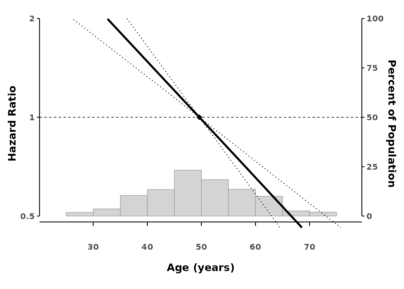
The plot shows: - The smooth effect of age on hazard - 95% confidence intervals (dotted lines) - A reference point (diamond) where HR = 1 - Histogram showing the distribution of data
Logistic Regression
For binary outcomes:
gam_logit <- gam(binary ~ s(age),
                 family = binomial(),
                 data = data)

splineplot(gam_logit, data,
          ylim = c(0.5, 2.0),
          ylab = "Odds Ratio")
#> Using 'age' as x variable
#> Using refx = 49.62 (median of age)
#> Warning: Removed 67 rows containing missing values or values outside the scale range
#> (`geom_line()`).
#> Warning: Removed 64 rows containing missing values or values outside the scale range
#> (`geom_line()`).
#> Warning: Removed 95 rows containing missing values or values outside the scale range
#> (`geom_line()`).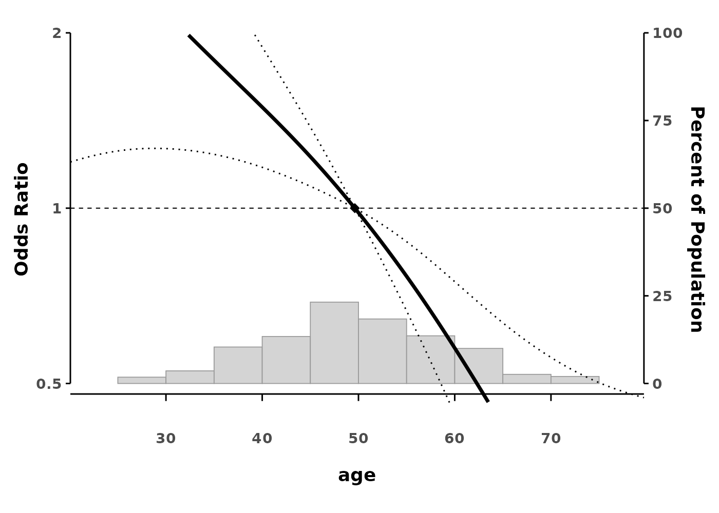
Poisson Regression
For count data:
gam_poisson <- gam(count ~ s(age),
                   family = poisson(),
                   data = data)

splineplot(gam_poisson, data,
          ylab = "Rate Ratio")
#> Using 'age' as x variable
#> Using refx = 49.62 (median of age)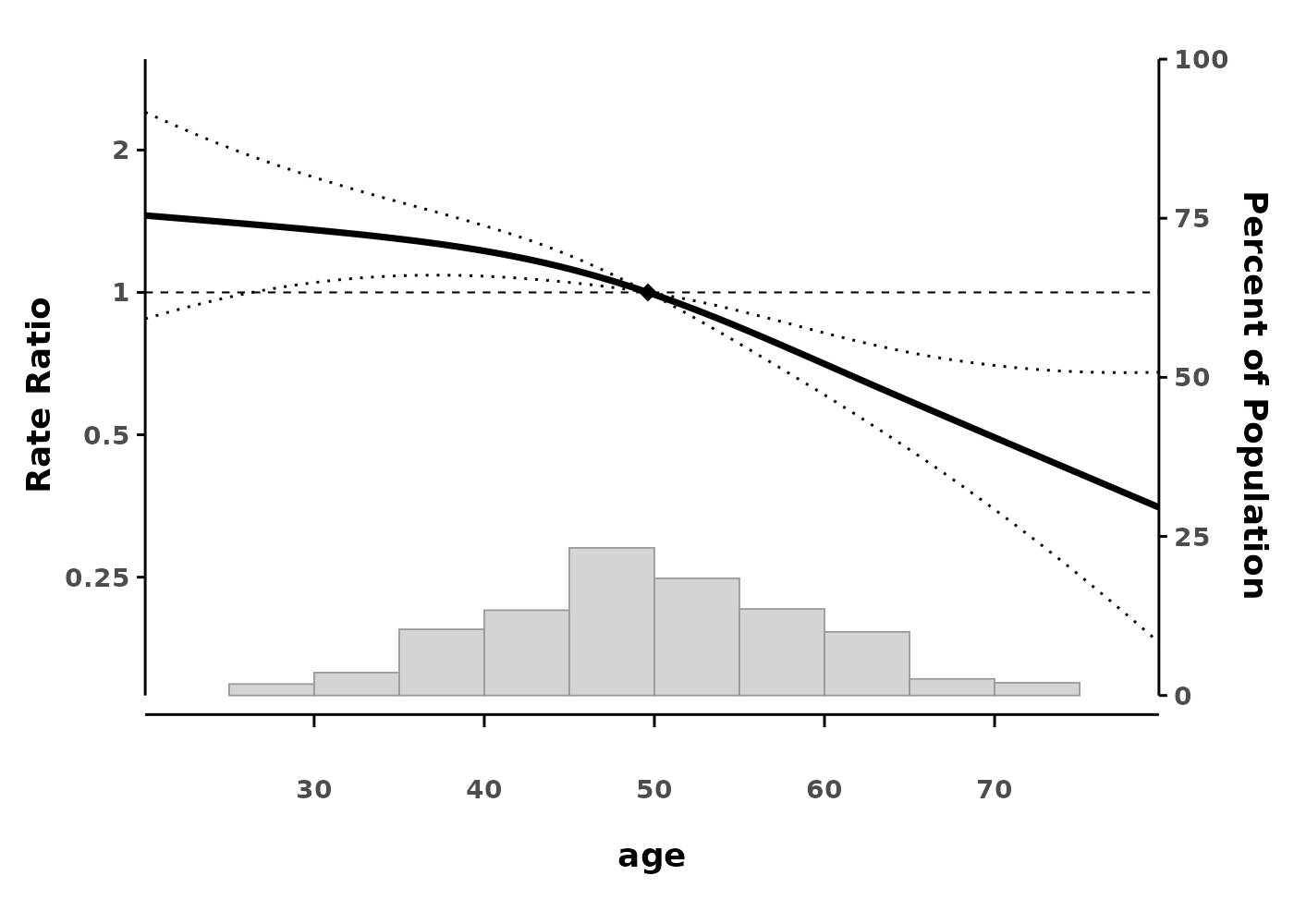
GLM with Splines
When you prefer parametric splines over GAM smooths:
Natural Splines (ns)
glm_ns <- glm(binary ~ ns(age, df = 4),
              family = binomial(),
              data = data)

splineplot(glm_ns, data,
          ylim = c(0.5, 2.0))
#> Using 'age' as x variable
#> Using refx = 49.62 (median of age)
#> Warning: Removed 77 rows containing missing values or values outside the scale range
#> (`geom_line()`).
#> Warning: Removed 72 rows containing missing values or values outside the scale range
#> (`geom_line()`).
#> Warning: Removed 88 rows containing missing values or values outside the scale range
#> (`geom_line()`).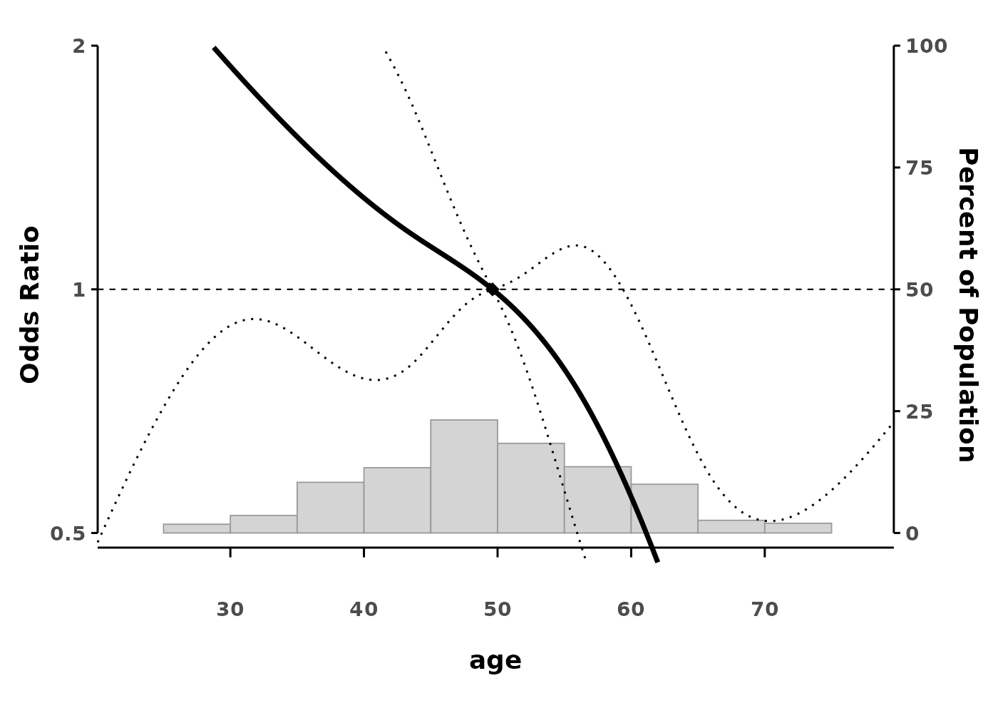
B-splines (bs)
glm_bs <- glm(count ~ bs(age, df = 4),
              family = poisson(),
              data = data)

splineplot(glm_bs, data)
#> Using 'age' as x variable
#> Using refx = 49.62 (median of age)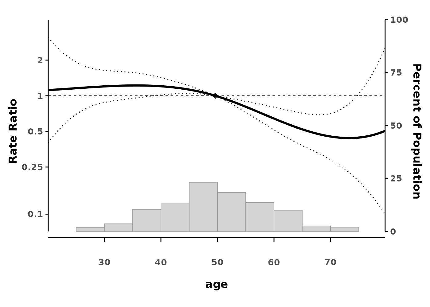
Cox Models with Splines
For survival analysis without GAM:
cox_ns <- coxph(Surv(time, status) ~ ns(age, df = 4),
                data = data)

splineplot(cox_ns, data,
          ylim = c(0.5, 2.0))
#> Using 'age' as x variable
#> Using refx = 49.62 (median of age)
#> Warning: Removed 92 rows containing missing values or values outside the scale range
#> (`geom_line()`).
#> Warning: Removed 50 rows containing missing values or values outside the scale range
#> (`geom_line()`).
#> Warning: Removed 93 rows containing missing values or values outside the scale range
#> (`geom_line()`).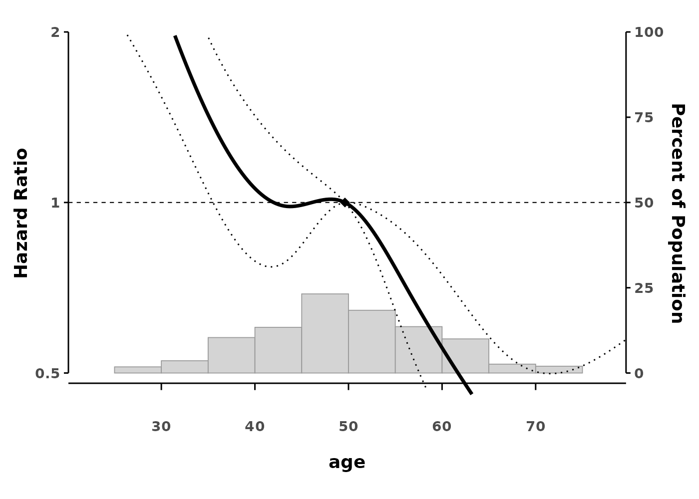
Customizing Your Plots
Reference Values
By default, the reference value is the median. You can change this:
splineplot(gam_cox, data,
          refx = 45,  # Set reference at age 45
          ylim = c(0.5, 2.0))
#> Using 'age' as x variable
#> Warning: Removed 71 rows containing missing values or values outside the scale range
#> (`geom_line()`).
#> Warning: Removed 67 rows containing missing values or values outside the scale range
#> (`geom_line()`).
#> Warning: Removed 79 rows containing missing values or values outside the scale range
#> (`geom_line()`).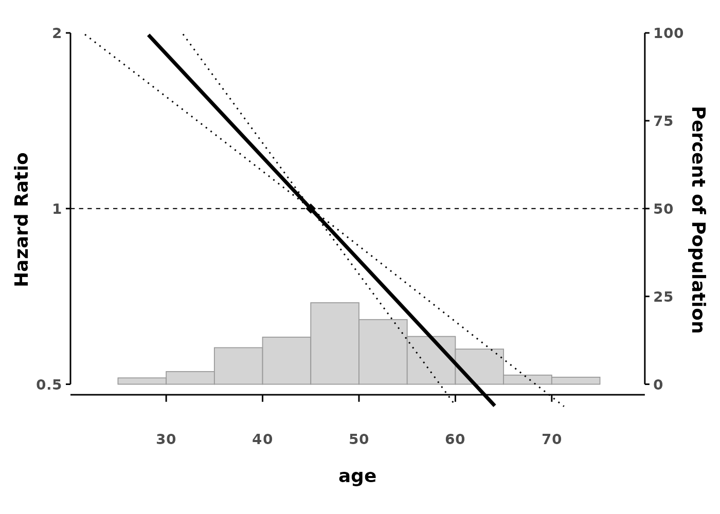
Confidence Interval Styles
Choose between dotted lines (default) or ribbon style:
# Ribbon style confidence intervals
splineplot(gam_logit, data,
          ribbon_ci = TRUE,
          ylim = c(0.5, 2.0))
#> Using 'age' as x variable
#> Using refx = 49.62 (median of age)
#> Warning: Removed 131 rows containing missing values or values outside the scale range
#> (`geom_ribbon()`).
#> Warning: Removed 95 rows containing missing values or values outside the scale range
#> (`geom_line()`).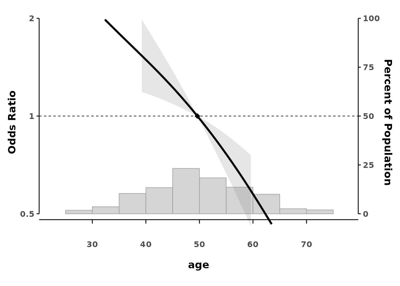
Histogram Options
You can toggle the histogram display:
splineplot(gam_cox, data,
          show_hist = FALSE,
          ylim = c(0.5, 2.0))
#> Using 'age' as x variable
#> Using refx = 49.62 (median of age)
#> Warning: Removed 71 rows containing missing values or values outside the scale range
#> (`geom_line()`).
#> Warning: Removed 67 rows containing missing values or values outside the scale range
#> (`geom_line()`).
#> Warning: Removed 79 rows containing missing values or values outside the scale range
#> (`geom_line()`).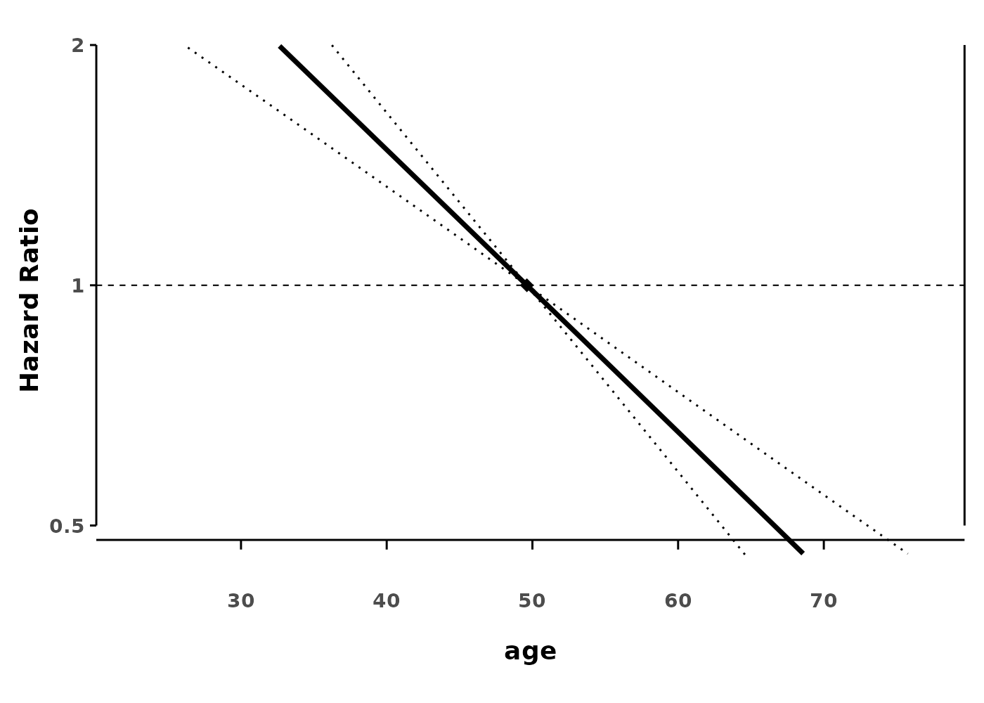
Log Scale
For odds ratios, rate ratios, or hazard ratios, you might prefer log scale:
splineplot(gam_logit, data,
          log_scale = TRUE)
#> Using 'age' as x variable
#> Using refx = 49.62 (median of age)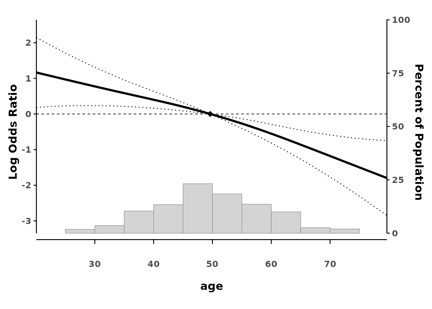
Interaction Terms
The package automatically detects and visualizes interaction terms:
# Add a grouping variable
data$group <- factor(sample(c("Male", "Female"), n, replace = TRUE))

# Fit model with interaction
gam_interact <- gam(time ~ s(age, by = group),
                   family = cox.ph(),
                   weights = status,
                   data = data)

# Plot shows separate curves for each group
splineplot(gam_interact, data,
          ylim = c(0.5, 2.0))
#> Using 'age' as x variable
#> Detected interaction with 'group'
#> Using refx = 49.62 (median of age)
#> Warning: No shared levels found between `names(values)` of the manual scale and the
#> data's fill values.
#> Warning: Removed 165 rows containing missing values or values outside the scale range
#> (`geom_line()`).
#> Warning: Removed 111 rows containing missing values or values outside the scale range
#> (`geom_line()`).
#> Warning: Removed 150 rows containing missing values or values outside the scale range
#> (`geom_line()`).
Tips for Best Results
- Model Choice: Use GAM for maximum flexibility, GLM with splines for parametric approach
- Degrees of Freedom: Higher df allows more flexibility but may overfit
- Reference Point: Choose a meaningful reference value for interpretation
- Confidence Intervals: Ribbon style is visually appealing, dotted lines show precision better
- Sample Size: Ensure adequate sample size for stable spline estimates