Population Genetics Index: 유전체역학 2017
개념설명은 https://www.slideshare.net/secondmath/fst-selection-index 을 참고하기 바란다.
Fst
Load package & Data Load
library(hierfstat);library(data.table);library(knitr);library(DT)
fst.file="https://raw.githubusercontent.com/jinseob2kim/jinseob2kim.github.io/master/fstexample.txt"
a=fread(fst.file)
Read example file. 7 pop & 289 SNPs (PER3 gene)
datatable(a) Basic stat: original Fst
gg=basic.stats(a)
perloc1=gg$perloc                       # per locus statistics
datatable(perloc1) %>% formatRound(1:ncol(perloc1),3)
fstloc1=perloc1$Fst # per locus Fst
all1=gg$overall # overall locus statistics
kable(t(all1),caption = "overall locus statistics",digits = 3)| Ho | Hs | Ht | Dst | Htp | Dstp | Fst | Fstp | Fis | Dest |
|---|---|---|---|---|---|---|---|---|---|
| 0.282 | 0.307 | 0.332 | 0.024 | 0.336 | 0.029 | 0.074 | 0.085 | 0.081 | 0.041 |
fst1=all1[7]                            # overall locus Fst
fst1
## Fst
## 0.074Weir & Cockerham’s theta
gg2=wc(a)
fstloc2=gg2$per.loc$FST                # per locus fst
kable(t(head(fstloc2)),digits=3,caption = "First 6 Fst")| 1 | 2 | 3 | 4 | 5 | 6 |
|---|---|---|---|---|---|
| 0.052 | 0.052 | 0.064 | 0.045 | 0.061 | 0.011 |
fst2=gg2$FST                           # overall locus: mean
fst2
## [1] 0.07931026Compare
library(ggplot2)
f=data.table(fstloc1,fstloc2)
ggplot(f,aes(fstloc1,fstloc2))+geom_point()+xlab("Wright's Fst")+ylab("Cockerham's theta")+annotate(geom="text", x=0.02, y=0.4,label= paste("r =",round(cor(fstloc1,fstloc2),3)),size=5)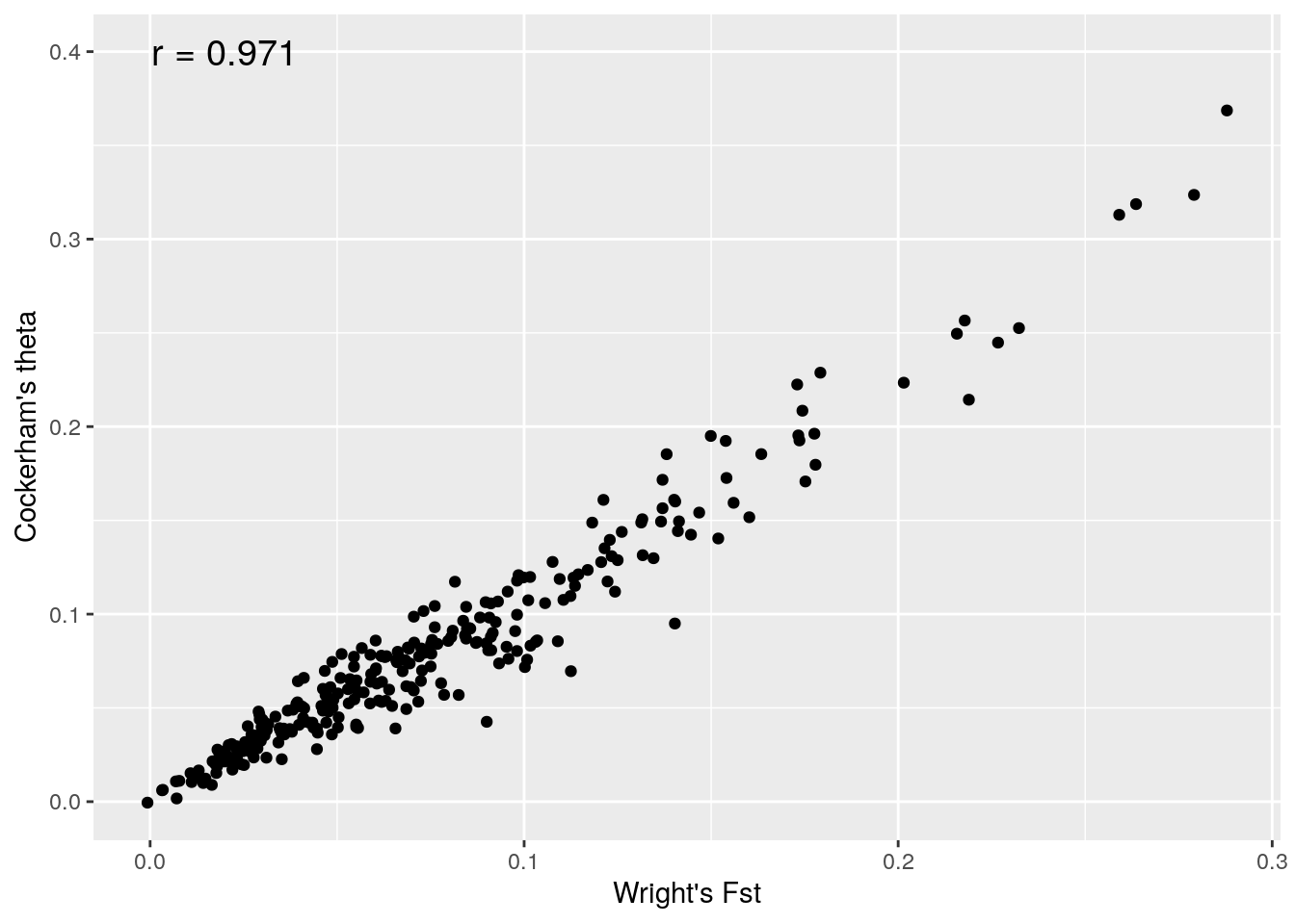
Selection Index: EHH, iHS, xpEHH
Read example file, chr=12: 1424 SNPs & 280 haplotype
library(rehh)
make.example.files()
datatable(fread("bta12_cgu.hap")[1:100],rownames = F)datatable(fread("map.inp")[1:100],rownames=F)b<-data2haplohh(hap_file="bta12_cgu.hap",map_file="map.inp",
recode.allele=TRUE,chr.name=12)## Map file seems OK: 1424 SNPs declared for chromosome 12
## Standard rehh input file assumed
## Alleles are being recoded according to map file as:
## 0 (missing data), 1 (ancestral allele) or 2 (derived allele)
## Discard Haplotype with less than 100 % of genotyped SNPs
## No haplotype discarded
## Discard SNPs genotyped on less than 100 % of haplotypes
## No SNP discarded
## Data consists of 280 haplotypes and 1424 SNPsBifurcation plot
bifurcation.diagram(b,mrk_foc=456,all_foc=1,nmrk_l=20,nmrk_r=20,
main="Ancestral Allele")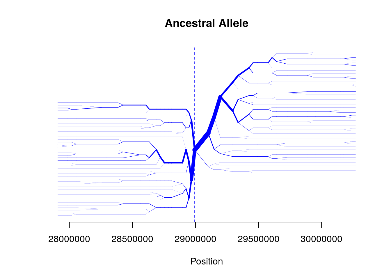
bifurcation.diagram(b,mrk_foc=456,all_foc=2,nmrk_l=20,nmrk_r=20,
main="Derived Allele")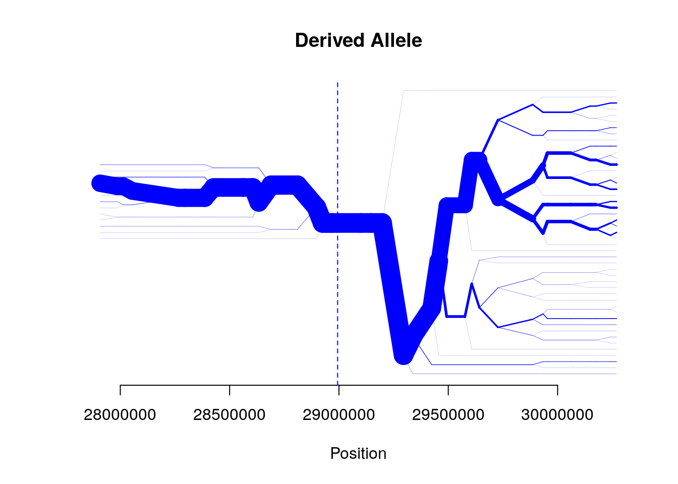
EHH, Site specific EHH(EHHs)
# computing EHH statistics for the focal SNP at position 456
#par(mfrow=c(1,2))
res1=calc_ehh(b,mrk=456,limhaplo=2,limehh=0.05,plotehh=T)
include_graphics("ehh.png")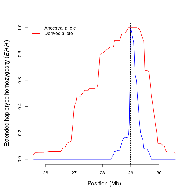
res11=calc_ehhs(b,mrk=456,limhaplo=2,limehh=0.05,plotehh=TRUE)   # site EHH
include_graphics("ehhs.png")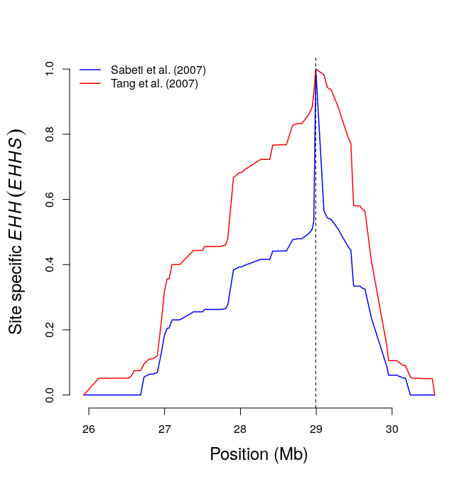
Integrated EHH
res2=scan_hh(b)                  # a: ancestral, d: derived, IES: average of IHHa & IHHd (squared allele freq weighted)
datatable(res2) %>% formatRound(3,2) %>% formatRound(4:7,0)
iHS
ihs_res2=ihh2ihs(res2)
datatable(ihs_res2$iHS) %>% formatRound(3:4,3)                       ## iHS & pvalue
datatable(ihs_res2$frequency.class) %>% formatRound(2:3,3) ## summary per alle freq bin.ihsplot(ihs_res2) ## iHS plot: y- pvalue, x-bp
include_graphics("iHS.png")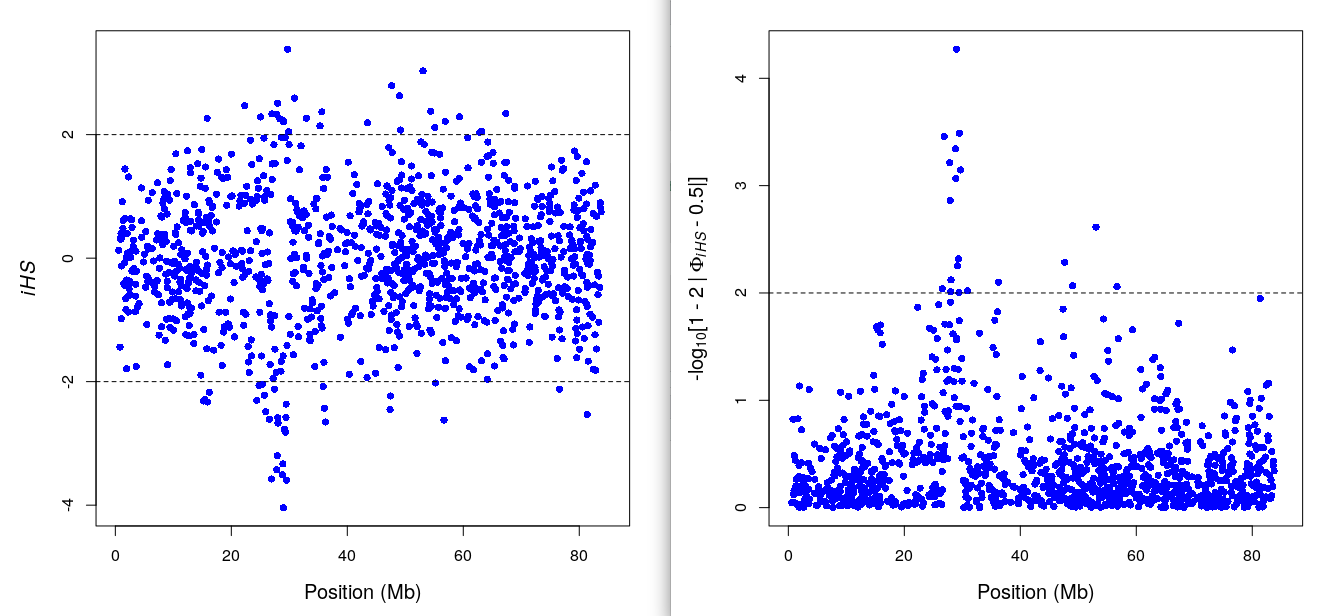
Population Comparison: rSB & xpEHH
data(wgscan.cgu) ; data(wgscan.eut)                 ## Load example result
res.rsb=ies2rsb(wgscan.cgu,wgscan.eut,"CGU","EUT")  ## Rsb: Compare 2 population
kable(head(res.rsb),digits=3)| CHR | POSITION | Rsb (CGU vs. EUT) | -log10(p-value) [bilateral] | |
|---|---|---|---|---|
| F0100190 | 1 | 113642 | -0.340 | 0.134 |
| F0100220 | 1 | 244699 | -1.057 | 0.537 |
| F0100250 | 1 | 369419 | -0.147 | 0.054 |
| F0100270 | 1 | 447278 | -1.819 | 1.162 |
| F0100280 | 1 | 487654 | -0.219 | 0.083 |
| F0100290 | 1 | 524507 | -0.794 | 0.369 |
rsbplot(res.rsb)                                    ## Rsb plot
include_graphics("rsb.png")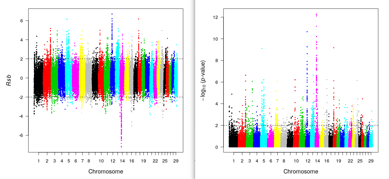
res.xpehh<-ies2xpehh(wgscan.cgu,wgscan.eut,"CGU","EUT")
kable(head(res.xpehh),digits=3)| CHR | POSITION | XPEHH (CGU vs. EUT) | -log10(p-value) [bilateral] | |
|---|---|---|---|---|
| F0100190 | 1 | 113642 | -0.556 | 0.238 |
| F0100220 | 1 | 244699 | -0.752 | 0.345 |
| F0100250 | 1 | 369419 | -0.889 | 0.427 |
| F0100270 | 1 | 447278 | -0.347 | 0.138 |
| F0100280 | 1 | 487654 | -0.918 | 0.446 |
| F0100290 | 1 | 524507 | -0.752 | 0.345 |
xpehhplot(res.xpehh)                                ## xpEHH plot
include_graphics("xpehh.png")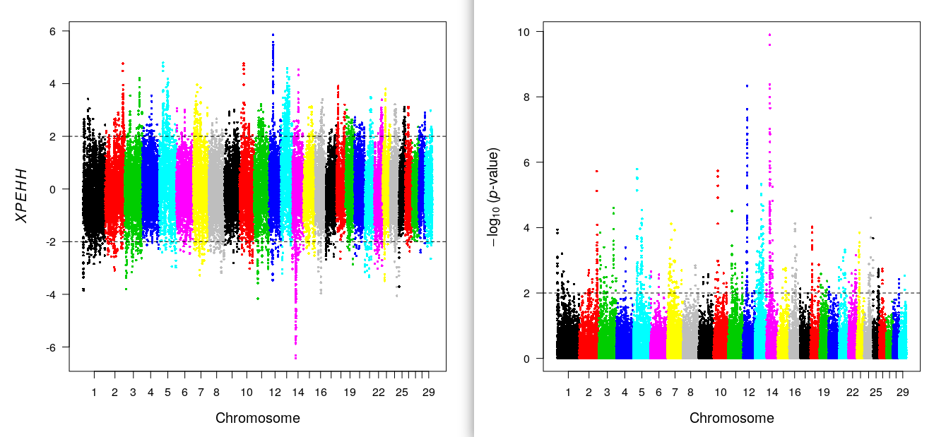
plot(res.rsb[,3],res.xpehh[,3],xlab="Rsb",ylab="XPEHH",pch=16,cex=0.5,cex.lab=0.75,cex.axis=0.75)
abline(a=0,b=1,lty=2,main="Rsb vs xpEHH")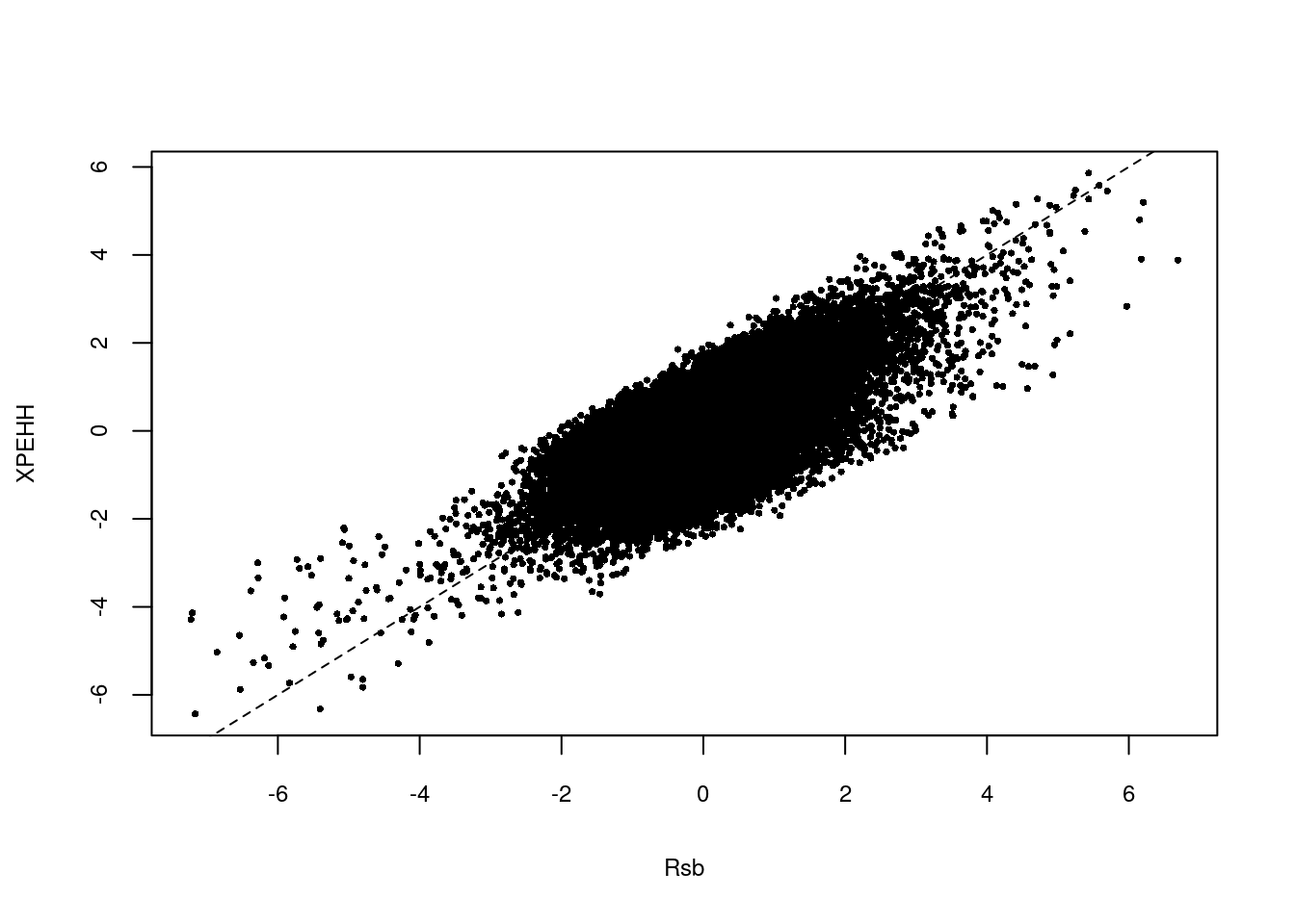
Copyright ©2016 Jinseob Kim